Rapid Bin Centres Frequency Response Analysis
Linked Resources:
| APPLICATION NOTES |
| QUICK STARTS |
| RELEVANT PRODUCTS |
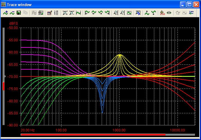
This series of 32 individual 64k-point frequency response curves took around 2 minutes to create
using the bin-centres method. Try that with swept measurements!
The dScope Series III is a powerful and comprehensive audio analyzer platform, designed to give the user a great deal of flexibility in analyzing audio signals and carriers, making the system ideally suited to a wide range of applications from R&D to production-line testing.
One measurement that is often used by engineers to characterise the linear behaviour of an audio device is a frequency response plot. dScope's flexibility affords the user a number of different options for analyzing frequency response, including:
- Sweeps (log / linear / custom distribution of points)
- Multi-tone frequency response (derived from FFT)
- FFT of Impulse response
- FFT of Bin-Centres multi-tone stimulus
The last case, the Bin-Centres method of analyzing frequency response, will be the focus for discussion in this article. This method produces a very high resolution frequency response, and executes very quickly - a complete frequency response is generated in the time taken for dScope to capture and process a single FFT buffer. This allows the user to see, for example, the effect of adjusting EQ settings in close to real-time, without the delays normally associated with running a sweep, changing the EUT circuit, repeating the sweep etc. As an example see the illustration above.
To highlight the potential speed of this method, a 4096-point, single-channel frequency response can be generated in as little as 150ms at 48kHz Fs (actual calculation time will depend on a number of factors including processor speed of host PC).
Theory
This method of achieving a frequency response in a very short space of time relies on two processes:
- Generating a very specific multi-tone signal to feed to the EUT input
- Analyzing the FFT of the EUT output
FFT - The Basics
We will not delve deeply into the mathematics of the FFT, but in simple terms, the FFT is a mathematical algorithm used to convert a time domain waveform into its equivalent frequency domain representation (spectrum). The input to the algorithm is a sequence of digitised time domain samples ('sample buffer'), where the sequence has a total length of 2n samples (where n is an integer). The output from the algorithm is a series of 2n frequency domain points, distributed linearly from 0Hz (DC) to the digital sample rate (Fs). This means that 2n / 2 points lie between DC and the Nyquist limit (Fs / 2) in the resulting output spectrum.
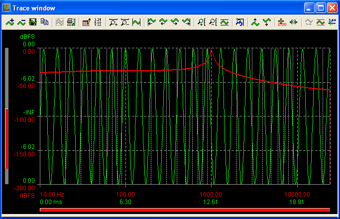
Figure 1: un-windowed 1024 point FFT of 1kHz sine wave
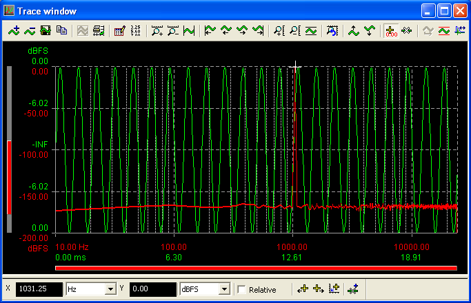
Figure 2: un-windowed 1024 point FFT of 1.03125kHz sine wave
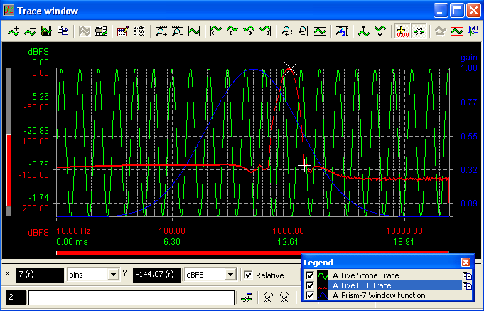
Figure 3: 1024 point FFT of 1kHz sine wave with Prism 7 window function (blue trace)
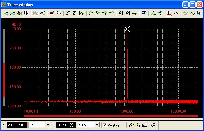
Figure 4: 256k point FFT of 1kHz sine wave with Prism 7 window function (16 frequency domain averages)
In employing the FFT algorithm, we have made the assumption that the time domain signal under analysis 'wraps' perfectly from the end of the sample buffer back to the beginning. You will notice that the time domain signal in Figure 1 starts at a positive-going zero crossing, and ends at around +9V just after a peak, which means it has a large discontinuity between the two ends of the signal. The FFT result displayed in Figure 1 clearly shows a distinct peak at the signal frequency of 1kHz, but this peak has a high amplitude 'skirt' over a very wide range of frequencies, giving poor resolution of the noise floor in the presence of the signal. This smearing is caused by the effective discontinuity in the time domain signal as the signal wraps from the beginning to the end of the buffer.
Figure 2 shows what happens if there is no discontinuity in the time domain buffer - here we have chosen a signal frequency of 1031.25Hz, which aligns perfectly with the 22nd bin frequency of the 1k FFT, a frequency which fits precisely 22 whole cycles of sinusoidal signal in the time domain buffer. Here we see that (after 8 cycles of FFT buffer averaging to smooth the noise floor), we have a perfect 'spike' at the signal frequency, with the FFT trace returning to the same amplitude as the noise floor at one bin either side of the signal frequency.
Time Domain Windows
In the context of audio signal analysis, it is unusual for us to encounter sinusoidal signals which happen to exactly coincide with an FFT bin frequency, so we rarely have the luxury of analysing signals with an FFT resolution as in Figure 2 without first applying what is known as a 'window function' (we see later in the context of the bin-centres frequency response method that sometimes we can use an FFT without a window function). We can almost entirely negate the problems that we saw in Figure 1 by the use of a time domain window. The theory is that rather than attempting to use a signal which has perfect continuity at either end of the time domain buffer, we instead modify the signal by applying an amplitude window. This amplitude window is designed to gradually attenuate the signal to zero amplitude at either end of the sample buffer - we force the signal to wrap without discontinuity by enforcing a zero amplitude condition at either end of the sample buffer. Figure 3 shows what happens to the FFT of the same 1kHz sine wave that we used in Figure 1 if we apply the blue time domain window before the FFT is calculated. In this case, we have a used a 'Prism 7' window function, the default window function used in dScope's FFT analysis.
We can immediately see three results of the window function used in the FFT trace of Figure 3:
1) The resolution of the signal compared to the noise floor has significantly increased compared to the un-windowed (or 'rectangular' window) signal used in Figure 1.
2) The signal has been 'smeared' in the frequency domain compared to the ideal FFT shown in Figure 2. The degree of the smear is related to the shape of the window function used. In this case, we are using the 'Prism 7' window function, which will cause the 1kHz signal to be smeared ±7 frequency domain bins.
3) The secondary effect of the smearing caused by the window function is seen in the spread of the DC content of the signal, which appears to result in an elevated noise floor below 1kHz - this is due to an apparent lack of data points below 1kHz; the 7th bin occurs at 281.25Hz therefore the DC content is spread up to this frequency.
Although beyond the scope of this article, different window functions exhibit very different effects on the FFT result, trading-off dynamic range and signal smearing. Prism Sound recommend using the Prism 7 window function for most applications, as this will give the highest dynamic range for analysis of signals which do not fall into precise FFT bin frequencies. Figure 4 shows a high resolution (256k) FFT of the 1kHz signal in Figure 3 (16 frequency domain averages, Prism 7 window function). This Figure clearly shows the immense power of the FFT process in being able to resolve very low level residual components - the odd harmonics of the signal in Figure 4 can be clearly seen, despite their amplitudes being in the region of -180dB relative to the fundamental tone.
Rapid Frequency Response Measurement Procedure
Now that we have discussed the basics of using an FFT to derive a spectral analysis, we can now discuss how this can be used to make a frequency response measurement of a EUT.
As we saw in the Figure 2, there is a potentially useful property of the FFT algorithm that results in a 'perfect' 1-bin-wide peak in the FFT output if the signal frequency applied to the FFT algorithm is precisely aligned with an FFT bin frequency (provided no window function is used). It is this property that enables us to make the rapid frequency response measurement we are aiming to achieve: If, instead of using a single sinusoidal tone as our stimulus, we use a signal that contains a sum of sinusoidal components centred at every FFT bin frequency over the bandwidth of interest, our un-windowed FFT will then give us the frequency response of the signal under test, as each point will be plotted discretely without smearing, giving us a perfectly smooth response curve.
This type of multi-tone signal is referred to as a 'Bin centres' stimulus in dScope, as the centre of every bin frequency in the FFT will be occupied by a single sinusoidal tone component. This is distinct from other types of more sparsely-populated multi-tone signals, which can be used to analyze a great deal more than just frequency response. More information on this type of multi-tone is available on the multi-tone applications page
The following procedure describes how to configure a bin-centres derived fast frequency response using dScope. Note that the 'Bin centres' generator signal is available from software version 1.2x onwards. The latest software can be downloaded from the dScope downloads page.
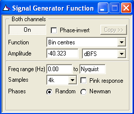
Figure 5: dScope's signal generator window
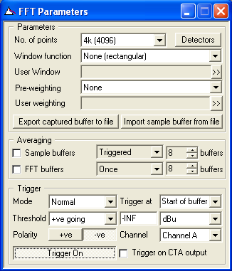
Figure 6: dScope's FFT Parameters window
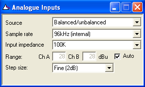
Figure 8: dScope's analogue Inputs window
If the EUT is purely analogue, this is already taken care of as dScope's analogue analyzer clock is synchronised to the analogue generator clock.
If your analysis is cross-domain or purely digital, you will need to synchronise your EUT to dScope (or vice versa), or if this is not possible, you may be able to use dScope's sample-rate-conversion window functions - you will need to specify this in the FFT parameters dialogue box in the 'Window Function' dialogue box (see section 3 below).
2) Configure the Signal Generator
You will need to select your signal generator function as 'Bin Centres' - see Figure 5. There are options for the signal amplitude and bandwidth, in addition to the number of samples in the generator sequence. Note that the signal amplitude refers to the amplitude of each tone component rather than the total signal amplitude. There are options for either random or Newman phase distribution - random will give a noise-type sound, and Newman will sound more like a fast swept sine (chirp). The advantage of the Newman phase response is that the crest factor is minimised, to provide better analysis signal-to-noise ratio. Pink-weighting will give the signal an amplitude response that falls at a rate of 3dB per octave with increasing frequency.
3) Configure the FFT Parameters
In order for the analysis to work correctly, you need to configure the FFT parameters (Figure 6) to contain the same number of points as per the length of the signal defined in the signal generator, and set the window function to 'None (rectangular)'.
Note that if you are making a cross-domain or purely digital analysis, and you cannot synchronise your EUT to dScope or vice versa, you can choose a sample-rate-converting window function to correct for any discrepancies in clock frequencies between the EUT and dScope.
Provided you have the FFT trigger switched on in 'Normal' mode (and assigned to an appropriate trigger condition), you should now see a continuously updating frequency response being displayed by the FFT trace in the trace window. If you wish to preserve a trace at any time, you can simply click on the appropriate copy curve icon in the trace legend and assign a new colour / name as you wish.
The resulting frequency response graph should look a little like those shown in the example at the top of the page - albeit the shapes of the response curves will depend on the nature of the EUT.
If you wish to see a static view of the time domain trace as the FFT result updates, you can assign the trigger mode to 'Generator Wavetable' in the FFT Parameters window - the sample buffer will then start to fill at the start of the signal generator sequence every cycle.
Trade-Offs and Further Information
The main trade-off with this method for analyzing frequency response is one of resolution versus speed. This FFT-derived result will result in a linear distribution of x-axis data points, therefore if you view the result on a logarithmic x-axis scale, there will be an apparent reduction in resolution as frequency decreases. In order to increase the low frequency resolution, a larger FFT size (and corresponding signal generator length) can be chosen. However, this increased signal length will take longer to acquire, and also longer to process, so the update rate for the FFT result will decrease.
As a typical example, for a single channel measurement at 48kHz Fs, you can expect to see a frequency response update somewhere between around every 0.1 seconds (1k FFT) and around every 6 seconds (256k FFT). Exact timings will depend on a number of factors, including the processor speed of the host PC.
A second trade off is resolution versus signal to noise ratio. A sinusoidal signal at 0dBFS will give maximal signal to noise ratio at that frequency. If the tone amplitude at 1kHz is lowered by, say, 40dB in order to accommodate the remaining tones within the 0dBFS limit of the system, the signal to noise ratio in the 1kHz bin will have reduced, and therefore the 1kHz multi-tone derived amplitude will be more susceptible to noise than the single-tone result.
This should not be a problem for most systems, but if very noisy systems are causing analysis problems, there are a number of adjustments that may be made to help reduce the influence of noise on the measurement:
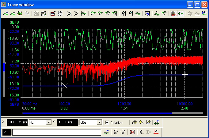
Figure 9 - EUT is clipping, giving red frequency response curve (clipped samples visible in green time domain trace, offset for clarity). Input level to EUT is reduced, giving blue frequency response curve.
- If the noise is worse at low frequencies, try selecting 'Pink Response' in the signal generator - the relative amplitude of the low frequency components will increase, thus increasing the signal to noise ratio in this band.
- If the noise is worse at high frequencies, select 'Newman Phase' in the signal generator to reduce the crest factor of the signal - this will increase the maximum amplitude you can use per tone component.
- Reducing the number of samples in the generator signal (and the corresponding FFT analysis) will allow a higher signal amplitude at each tone frequency.
- Reducing the bandwidth of the generator signal to cover only the range of frequencies you are interested in analyzing will also reduce the number of tones used, and therefore enable a higher amplitude for each tone.
- Switching on Sample Buffer Averaging in the FFT Parameters window (Figure 6) will average out the effect of unwanted noise, albeit with the obvious penalty of a longer calculation time for each frequency response result.
- If the EUT is an electro-acoustic system, consider using impulse-response analysis as discussed in the impulse response application note, which can generate results almost as quickly as the bin centres method.
In order to ensure optimal use of the full range of dScope's analyzer ADC, it is important to ensure that the analogue gain ranging is set to the most sensitive setting possible when analyzing analogue signals. Figure 8 shows dScope's Analogue Inputs dialogue box. For sinusoidal signals, the gain ranging can be left in 'Auto' mode with a 'Fine (2dB)' step size. However, with a signal which has a crest factor higher than that of a sine wave (such as the 'Bin centres' stimulus discussed in this article), these settings may not be suitable - if the signal amplitude varies significantly over the duration of sample buffer capture, the gain ranging may switch amplitudes mid-buffer capture, causing the capture to re-start, and the analysis to fail (repeatedly, if analysis is continuous).
If the sample buffer fill is failing, and / or you can hear the analogue gain ranging relays latching, you will need to enter a fixed analogue amplitude range, slightly higher than the maximum amplitude of the signal under test, or opt for a less sensitive step size in the auto gain ranging. The latter case may still cause problems if the 'Fine' gain step which is causing a problem happens to coincide with a 'Medium' or 'Coarse' gain step.
EUT Overload
It is important that the EUT inputs / outputs are not overloaded - if the input signal amplitude is too high, the resulting output spectrum will include a large quantity of distortion components in addition to the signal components. This will result in a very 'noisy' looking frequency response - see Figure 9. The solution is to reduce the input level / gain of the EUT until a smooth response is obtained.
Conclusion
We have presented and discussed a very fast method for analyzing the frequency response of a EUT, without the need to run a swept measurement. This method can give very high resolution output, and execute very quickly compared to a similar resolution sweep. This rapid analysis lends itself well to highly repetitive tasks, including production line analysis and characterising devices with many different frequency response settings. Some inter-related trade-offs concerning low frequency resolution, analysis speed and signal to noise ratio have been discussed in detail, and should give the user sufficient information to configure this type of result for a wide range of EUTs.
For further technical information on this, or any other aspect of dScope's analysis capabilities, please contact us using the form below.
App ID: 0020, Resource ID: 90